Cocept of supply

Supply like demand is also function of price.It is expressed as,S=f (P) :When the price the price of commodity changes,the supply of the commodity changes.But unlike demand,supply varies directly with price.The supply has positive relationship with price.It implies that supply increase in price.The supply is the quality that a seller is willing to sell at particular price and particular time.
According to Watson and Getz-"In economics,the word supply always means a schedule-a schedule of possible prices and of amount that would be sold at each price."
According to R.C.Lipsey -"The amount of a commodity that firms are able and willing to offer for sale is called the quality supplied of that commodity."
The concept of supply curve is relevant only in perfectly competitive market.The nation of supply curve is not applicable in other forms of market like monopoly,monopolists.Because the main task of a supply curve is to show much a firm can supply at the given price.In perfect competition,a firm is only a price-taker and quantity-adjuster price.In the imperfectly competitive markets,a firm determines the price of its product.It is not necessary to adjust supply at given price.

Revenue curves

There are 2 types of revenue curves :

1. Concept of total revenue,average revenue and marginal revenue :A firm earns revenue by selling its products.The revenue earned by it is divided into 3 parts-total revenue and marginal revenue.

• Total revenue :The total earned by a firm by selling its product is called total revenue.The total revenue is obtained by multiplying price per unit of a commodity by the total quality sold.Hence,it is expressed as ,

TR=P*Q
Where TR=total revenue,P=price and Q=quality.As for average example,if 10 units of a commodity are sold at price rs.10.per unit,TR=rs.10*10=rs100.

• Average revenue :The average revenue is the price per unit of a commodity.The average revenue is obtained by dividing total revenue by the total quality sold.Hence,it is expressed as.

AR=TR/Q
Where AR=average revenue.As for example,if total revenue is Rs.100 and total quantity sold is 10 units,
AR=100/10=Rs.10.
The question crops up whether the average revenue and price are same thing?The answer is that if different units are sold at the same price,average revenue and price are equal.But if different units are sold at different prices,the average revenue and price are not equal.However in real life,different units are sold at the same price.Hence,in economics average revenue is synonymous with price.It is to be noted that the average revenue curve of a firm is the demand curve of a consumer.Since the demand curve shows the quantities demanded at different prices,it also shows average revenue of a firm.Because ,the price paid by a consumer is the revenue from a seller's viewpoint.

• Marginal revenue :The marginal revenue is the addition made to total revenue while selling one more unit.According to C.E.Ferguson "Marginal revenue is the change in total revenue associated with the change in one unit of output."It is expressed as.

2.Derivation of AR and MR curves from TR curve:The average revenue and marginal revenue curves can be obtained from total revenue curve.The process is little bit different in perfect competition and monopoly or imperfect competition.Because price remains constant under perfect competition.On the other hand,price is reduced to sell more quantities under monopoly.
3.Revenue curves under perfect competition :The demand curve of a firm under perfect competition is perfectly elastic.The price is beyond the control of a firm.Because price is determined by the industry as a whole.The average revenue or price thus remains constant.If different units are sold at same price,marginal revenue equals price.

Shape of LAC curve:Empirical envidence

According to the traditional theory,the long-run average cost curve is also 'U' shaped like the short run average cost curve.But some economists have found from empirical study that the LAC curve is L shaped rather than being 'U' shaped .The LAC curves first fall rapidly in the beginning.But after a point it becomes fully flat or may slopes downward slowly.Such a L shaped LAC curve is shown in figure below.
According to most of the empirical studies there is increasing returns to scale in lower level of production.But when output increases,the economies of scale decline and the consist returns to scale operates in higher level of production.This implies that as the output increase,the LAC curve slopes downwards at the diminishing rate and finally becomes horizontal.The operation of decreasing returns to scale or output of average cost curve is rarely found.
P.J.D.Wiles has concluded on the basis of his that the average cost like the branch of left side of capital letter 'U' first rapidly and then slowly slopes downwards.The decline in cost with size is almost universal.But 'U' never turns upward.The rapid increase in cost with size is practically unknown and even little rise as rare.He remarks"Most of the cost function obey what we may call the L-shaped costs."Johnston has also derived same conclusion from his study.From the study of cost estimate of electricity production in Great Britain,he has found the average cost to decline in the beginning and then becoming leveled off.
The reasons for the LAC curve being L shaped are as follows :

1. Technological progress :In economics theory,technological is assumed to be constant.But technology changes in real life.Due to this,the average cost decline and does not rise.Suppose that the firm in the beginning produces quality at cost on working at curve.If we connect the minimum point of long run cost curve which is lower than average cost.
2. Learning by doing :The LAC curve completely slopes completely downwards due to learning by doing.Since the efficiently of firm increases due to continuing the work,it is able to reduce cost.As the output is increased,there is not only the increase in knowledge of many things,there is also an improvement in the management of plant.Due to this LAC curve is L shaped.
3. Management technique :According to the modern management theory,appropriate administrative structure is available to operate the plant of each size.There exists appropriate management technique in different levels of management.The management technique is available in large and small size.The cost of different management first fall up to certain plant size.The managerial cost slowly increase slowly up to very large level of output.
   

Diseconomies of scale

According to the traditional theory,due to the dis economies of scale after some level output,the LAC curve slopes upwards.The dis economies of scale occurs due to the human and behavioral problems in managing big business.The causes of dis economies of scale are as follows:

1. Managerial inefficiency :The manager cannot manage and coordinate efficiently if the production is made on a very large scale.The management becomes complimented,the managers become too busy and become less efficient in decision making.Due to this when the size of the firm or output increase,the staffs increase more than proportionately and the management becomes less efficient.This increase cost of production.The inability to collect monitor information in large scale production by top administrator has been called 'control loss' by Oliver Williamson.The existence of dis economies of scale has been denied by some economies.But such dis economies can be clearly seen in some industries.
2. Problems of moral and motivation:There is the problem of moral and motivation among both management and labour force in large scale production.The collective feeling is less in firms than in small firms.The moral towards the organization is less is large firms.There is no incentive to increase production.The managers of large firms fell more secure and fell no fear of getting sacked.This makers them lethargic and devoid of entrepreneurship.Consequently,the cost of production increase.

Shape of LAC curve:Theoretical reasons

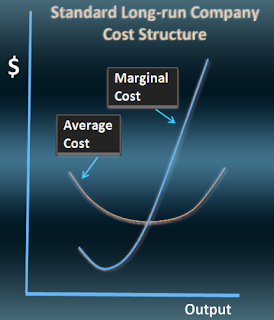
According to traditional theory the long run average cost curve (LAC) is also 'U' shaped.The operation of the laws of returns to scale is its main reason.In the beginning,there is the operation of increasing returns to scale.After the cost becomes minimum,there is the operation of decreasing returns to scale.Due too economics of scale and dis economies of scale,first the average cost falls and them rises.

Economies of scale :There is economies of scale when output in increased.The causes of economies of scale are :

1. Specialization :The specialization in the use of labour brings economies of scale.More the output,more the specialization of labour.This increases efficiency of labour.The labour productivity is higher i n large firms.This reduces unit cost of production in higher level of output.
2. Technological factors :The economies of scale also occurs due to technological factors.In large scale production highly specialized machinery and equipments can be used.The productivity of equipments rise rapidly more than cost.Due to this average cost decreases at higher level of output.According to Austin Robinson,the big machinery have the quality of integration of processes,the use of which brings economies of scale.The big automatics transfer or numerically controlled machinery can operate consecutive processes as well.From this there is saving in labour and time required in installing each plant.
3. Quantity discount :The existence of quantity discount also brings economies of scale.The quantity discount is available when raw materials and other factors it will be purchased in large quantity.The large firms can easily enter into capital and time market.They can get credit at lower rate of interest.This reduces the cost of capital.
4. Invisibilities :There is economics of scale due to fact that some factors are indivisible even in the long run.Due to indivisibility,the cost decrease until it reduces the full capacity.For example,management is indivisible even in the long run.In also proprietorship,he is fully indivisible.Due to this there is difficulty in management after a point.Even if all factors are divisible,there is economies of scale when the output is increased due to factors like division of labour.Due to this the per unit cost is lower in the long run.
   

Long run cost curves

The long run is a period of time when firms have sufficient time to change size of the plant and scale of operation.Since there are no fixed factors and fixed in the long run,there no fixed cost curves.All the factors are variable in the long run.Hence,we need to examine only long run average and marginal cost curves.The calculation of both these costs same as in the short run.It should be noted that the concept of long run cost is only hypothetical.Because,there can be no change in plant every now and them.

Derivation of long run average cost curve:In the short run,firm is tied to given plan.So there is only one average cost curve.But in the long run,the firm can change plant size.The large plant is used to produce more and the small plant is used to produce less.Hence,in the long run there may be many average cost curves.The firms produces at lowest average cost in long run than in the short run.
The long run average cost curve is derived from short run average cost curves as shown in the diagram.Suppose,there are three plants available-small,medium and large represented by SAC1,SAC2 and SAC3.
If a firm begins form small plant SAC1 and the demand for the product increase.It can produce output up to ox1 at lower cost.After this the cost increase.If demand reaches ox2,the firm can either continue production small plant or install medium plant represented by SAC2.If demand exceeds ox2,the firm installs medium plant.Because,the output more than ox2 can be produced at lower cost by medium plant than by small plant.
Similarly,the demand exceeds ox3;the firms installs large plant.Because,the output greater than ox3 can be produced at lower cost by large plant.the thick portion of each SAC curve thus shows the lowest long run average cost curve of producing particular level of output.Hence,the scallop shaped thick part of the short run average cost curves is long run average cost curve of the firm.

Detailed reasons

The further reasons for the short run average cost curve being 'U' shaped are as follows:

1.Economies of scale :Alfred Marshal has divided economies of scale into two parts internal economies and external economies.The internal economies arise due to the expansion of the first itself.On the other hand external economies arise to the expansion of the industry as a whole.The internal economies are of following types:

• Technical economies :The technical economies arise from the division of labour and economies in the use of plant and machinery.The division of labour increase efficiency which reduces per unit cost.Similarly,the use of large machinery reduces per unit cost when output is increased.
• Marketing economies :The marketing costs does not very with increase in sales up to certain point.So there is economies is purchase,transport,advertisement when sales increase.
• Managerial economies :The managerial cost decrease as the output increase.This is called managerial economies.A single manager can supervise large production up to certain limit.due to these economies of scale average cost decrease as the output increase.So AC curve is downward sloping in the beginning.This view has been seconded by a most of economists including Chamberlain.

2.Invisibilities :Some of the factors are indivisible such as machinery.The machinery or a manager cannot be cut into half to reduce output.So when the output is increased,these factors are efficiently utilized.This view is held by a host of economies including kanldo,Robinson,Stigler.

3.Law of variable proportions: According to the law of variable proportions if more and more variable factors are used to affixed factor,first the marginal product increases,but after a point,the marginal product declines..In other words,first the cost fall as the output is increased and after point cost increase as the output is increased.In the first stage of production.

Reasons for the 'u' shapes of short-run AC curve

The average cost curve of a firm in the short-run is 'U' shaped.The reasons for the 'U' shape of the short average cost curves are as follows :

1. Simple reason :The short run average cost curve is 'U' shaped due to nature of AFC and AVC curves as explained below.

• Fixed cost:The fixed cost is a constant quantity.The firm will have incur fixed cost even if the output is zero.Hence,the average fixed cost continuously fall as the output rises.On account of this,the average cost falls when output rises.
• Variable cost :The average variable cost varies with quantity output.In the beginning the average variable cost declines when the output increase.But beyond normal capacity,the average variable cost increase sharply.More output can be produced with more variable cost.With increase in output there is problems of over crowding,frequent breakdown of machinery.Consequently,average cost curve rises upwards as shown in the figure.
  

Derivation of short-run average &marginal cost curves

The derivation of short-run average and marginal cost curves an be explained by following elements:

1. Average fixed cost:The average fixed cost can be obtained fixed cost curve.It slopes downwards to the right.As the output increase,the ratio of fixed cost to output decreases.Because,the fixed cost is a fixed quantity.The AFC curve is a rectangular hyperbola.The AFC approaches both the axes but does not touch them.
2. Average variable cost:The variable cost per unit of output is called average variable cost.The average variable cost declines up to the normal capacity.The decrease in AVC in the beginning is due to the operations of law of diminishing returns.After normal capacity,the AVC increase rapidly.The AVC curve in figure represents average variable cost.It slopes downward in the beginning,reaches the minimum point and rises upward thereafter.In general,the AVC curve is'U' shapes.
3. Average total cost :The average total cost is,in fact only average cost.It is the cost per unit of output.The average total cost is obtained by dividing total cost by quantity of output.Alternatively,it may be obtained by adding average fixed cost and average variable cost.ATC is the average total cost.In the beginning,both AFC and AVC fall.So ATC falls rapidly.So ATC continue to fall.But if production is further increased.AVC increase rapidly.Hence,ATC rises after a point.In this way,ATC first falls,reaches minimum point and rises thereafter.Thus the ATC is almost 'U' shaped.
4. Marginal cost:The marginal cost is the addition made to total cost when one more unit is produced.The marginal cost of 2 units of output is obtained by subtracting the total cost of one unit of output from two units of output produced.The marginal cost is the change in total cost due to the change in output.Hence,it is also calculated as :

MC=TC/Q
The marginal cost is independent of the fixed cost.Because the fixed cost does not change with output.The total cost changes due to change in the variable cost.Hence,the marginal cost is also calculated as:
MC=VC2-VC1
As shown in the figure,the marginal cost first,reaches the minimum point and increases thereafter.Hence,the MC curve also first slopes downward,reaches the minimum point and rises thereafter.

Short-run total cost curves

The short run total cost can be explained as follows :

Fixed cost:The fixed cost is also called overhead cost,supplementary cost.The cost incurred in fixed factors is called fixed cost.The fixed cost cannot be changed in the short run.The fixed cost will have to be incurred even if the production is stopped for some time.The expenditure made on machinery,land,building and so on is the example of fixed cost.The curve representing these costs is called fixed curve cost curve.The sum of implicit fixed costs is called total fixed cost.The curve representing this is called total fixed cost curve.

Variable cost:The variable cost is also the prime cost,special cost and direct cost.The expenditures made on variable factors is called variable cost.The variable cost varies with output.The expenditure made on raw materials,wages,fuel are the examples of variable cost.The sum of the expenditures made on variable factors is the total variable cost.The curve representing this is called total variable cost curve.

Total cost:The sum of total fixed cost and total variable cost is total cost.Hence,TC=TFC+TVC.The total cost directly varies with output.Hence,the total cost is expressed as,TC=f(q),where q=quantity of output.The curve representing total cost is called total cost curve.

Fixed and variable costs

The costs that do not with output are defined as fixed costs.These costs will exist even if no output is produced.For example,interest on borrowed capital,rental expenses on leased plant or building,depreciation charges associated with the passage of time,salaries of employees who cannot be laid off during periods of reduced output are fixed costs.On the other hand,costs that very with changes in output are known as variable costs.They are function of the of output level.For example,expense on raw materials,wages,depreciation associated with the use of equipment,sales commissions,and the costs of all inputs that very with output are variable costs.Since all the factors are variable in the long run,so are all costs.
Such a sharp distinction between fixed and variable costs is not always realistic.For example,a salesman's salary might be fixed within a certain range of output,but below a lower limit he might be land off,while above the upper limit additional salesman would be hired.This problem led to the development of semi-variable cost concept.The semi-variable costs are fixed if incremental output does not exceed certain limits,but are variable outside these bounds.
The distinction between these cost concepts is useful in decision making.For example,in the short run a profit maximising firm will continue its operation so long as its total variable cost is covered but in the long run all costs must be covered.

Actual or outlay or costs and opportunity costs

The costs that are generally recorded in the books of account is called the actual costs.They consist of actual expenses of hiring land,labour,capital and management.The opportunity costs is the alternative that has been foregone.The opportunity cost of any good is the next best alternative good that is sacrificed.For example,the factors which are used for the manufacture of car may also be used for the production of military equipment.Therefor,the opportunity cost of the production of car is the output of the military equipment foregone.

The returns which the entrepreneur could have earned in an alternative use of his services and capital is called opportunity or alternative cost.Since the opportunity cost is a national cost,they are not recorded in a book of account.But they are useful for the purpose of decision making.The opportunity cost concept applies to all situation where a thing can have alternative uses.If there are no alternative,the opportunity cost will be zero.If alternative uses are many,the earning in the next best use will be the opportunity cost.According to Pappas and Brigham-"The alternative cost concept,then,reflects the fact that all decisions are based on choices between alternative actions.The cost of resource is determined by its value in its best alternative use."

Concept of costs

It is proper examine the different cost concepts which are useful in managerial decision making :
Accounting costs economics costs:The entrepreneur pays for the factors employed in production in the form of wages,interest,rent, and prices for raw materials,fuel and power.All these are included in cost of production.An accounting will take into account only the payments and charges made by the entrepreneur to the suppliers of various productive services.
The economist's view of cost in different.The entrepreneur invests his own capital,time,managerial talent in business.In the absence of his own business,he would have employed his resources in others business and benefited.The economists,therefor,includes in his cost of production the normal return on money capital invested by the entrepreneur him self and the wages or salary he cloud have earned inf worked for others.Likewise,money rewards for the factors owned and employed in his own business are also included by the economists in the cost of population.
Thus,accounting cost is the costs that cash payments.Economic costs consists of not only all accounting costs but also money on capital,service and mother factors the entrepreneur could have earned if he had invested in next best alternative uses.The accounting costs which is on contractual cash payment made by the firm to factor owners is a also called the explicit cost.On the other hand,the payments made for own service and factors is called implicit or imputed costs.The managerial decision making should be based on economic costs since the economic costs show the real cost of production of a project.

Assumptions of indifference curve

The theory of indifference curve is based on the following assumptions:

1. Not measurable quantitatively :Since utility is a psychological phenomenon,it cannot be measured quantitatively.
2. Levels of satisfaction comparable :The consumer can compare the different levels of satisfaction.But he cannot express the utility in particular quantity.
3. Consistent ranking :The consumer can rank his preference consistently.In fact,the basis of indifference curve is the preference indifference hypothesis.So if there are combinations A,B,C,D the consumer can rank their scale of preference.In indifference curve,the consumer can say whether he prefer A to B or B to A or is indifference between them.
4. Transitivity :Indifference curve assumes transitivity of preference.The transitivity means that if the consumer prefers A to B and B to C,he also prefers A to C.Similarly,if he is indifference between A and B and B and C,he is also indifferent between A and C.
5. Weak-ordering :Indifference curve is based on the weak ordering of the preference hypothesis.According to weak-ordering,the consumer may prefer A to B or B to A or he may be indifference between A and B.On the other hand,strong ordering assumes only that the consumer prefers A to B or B to n A but does not assume that the consumer can be indifferent between A and B.The strong ordering assumes the relation of preference.On other hand weak ordering assumes the relation of preference and also indifference.
   

Cardinal vs ordinal utility analysis

The concept of indifference curve was propounded in economics to replace the law of diminishing marginal utility.Marginal utility analysis is cardinal utility analysis and indifference curve analysis is ordinal utility analysis.These two concepts seen to be alternative.But,in reality,indifference curve has adopted some of the assumption of cardinal utility analysis.According to Edwin Marshal :The great 19th century economists like William Stanley jevons of England,Karl Menger of Austria,Leon Walras of France believed utility was measurable in cardinal sense.In contrast,most 20th century economists following the lead of E Slutsky,Vilfredo Pareto,Sir John Hicks assume that utility is measurable in an ordinal sense,Which means that a consumer can only rank various market baskets with regard to the satisfaction they give him and her."
The basic difference between marginal utility analysis and indifference curve analysis are as follows :

1. Measurement of utility :According to cardinal analysis,utility can be measured quantitatively.For example,the total utility derived from a commodity can be expressed as 20,30,40 units.Marginal utility can also be measured in similar way.But according to indifference curve analysis utility cannot be measured quantitatively,since utility is a psychological phenomenon.
2. Express the preference :According to cardinal analysis,utility can be measured quantitatively.So a consumer can express his preference.He not only can say that commodity X is preferable to Y,but he can also say by how much he prefers commodity X to commodity Y.But in ordinal utility,the consumer does not state quantity,but can say that the satisfaction derived from a combination of goods in high or low that from other combinations.
3. Interest in combination of goods :In cardinal analysis,it is assumed that a consumer becomes interested in a good in a particular period of time.Hence,most of its theories are based on the analysis of one commodity.But in ordinal analysis,it is assumed that the consumer is interested in a combination of good.He may prefer one combination to other or both combinations may be equally preferable to him.He is said to be indifference between two combinations.The curve on which combinations of goods yielding same total shown is called indifference curve.
4. Observe the preference :According to cardinal analysis,utility can be measured and at the same time the preference of the consumers can be observed.For example,if a man buys orange and does not buy apple,we can be say that he prefers orange to apple.According to ordinal analysis,utility cannot be measured,but it is possible to observed the preference of the consumer.For example,if a consumer spends all his money on combination A instead of combination B,we can say that he prefers combination A to B.Alternatively,we can say that he derived more satisfaction form combination A than from combination B.
   

Development of concept of idifference curve

Indifference curve is one of the important concepts of utility analysis.This concept has given shape to the theories of utility analysis.The evaluation of the concept of indifference curve cam be explained as follows:
First stage :In the first the credit for explaining the theories of utility analysis goes to Gossen (1854),Jevons (1871) and Walras (1874).The utility theories of these economists were fully developed by Alfred Marshall.
These economists regarded utility as a measurable quality of any commodity.Utility further assumed to be an additive quality and utility derived from one good is not affected by the rate of the consumption of another commodity.
Second stage :In the second stage,the theories of utility analysis was developed by Edgeworth (1881),Antonelli (1886) and Irving Fisher (1892).These writers also assumed that utility is a measured quality.
Final stage :Vilfredo Pareto (1906) developed indifference curve as an alternative approach.But his basic approach was same as that of second phase economists "These is only a change in interpretation,but is very important because it enable later writers to develop the theory of consumer behavior without resort to the assumption that utility is cardinally measurable."He did not assume cardinal measurement of utility.W.E.Johnson like Pareto expressed the view that the theory of consumer behavior need not be explained on the basis of cardinal measurement of utility.